I’ve been reflecting a bit on the global Covid-19 situation for the last couple of weeks, and I fear government failures around the world. The world governments’ reaction to the novel Coronavirus risks pushing our economies into a deep global recession. There is often an enormous cost to “an abundance of caution”. Are the risks worth the trade-offs?

The recent statement last week by the World Health Organization, claiming that 3.4% of those who caught Covid-19 died, is in all likelihood a gross upward bias of the true mortality rate. In South Korea, a country that has been hit particularly hard by the infection, the authorities there have administered more than 1,100 tests per million citizens. Analysis of their data suggests a mortality rate of 0.6%. As a point of comparison, the seasonal flu has a mortality rate of about 0.1%. High mortality from early estimates of Covid-19 seem to result from extreme truncation – a statistical problem that is not easy to solve. People who present themselves at medical facilities tend to be the worst affected making observation of those individuals trivial, while those who have mild symptoms are never heard from. Covid-19 is probably more dangerous than the flu for the elderly and those with pre-existing conditions which is almost certainly the main driver of the higher mortality rate relative to the seasonal flu. Italy’s numbers seem to be an outlier, but it’s unclear exactly what testing strategy they are using. At any rate, what worries me is not Covid-19 but the seemingly chaotic, on-the-fly world government responses that threaten to turn a bad but manageable problem into a global catastrophe. We have a precedent for such government policy failures in the past: The Great Depression.
In the late 1920s, in an attempt to limit speculation in securities markets, the Federal Reserve increased interest rates. This policy had the effect of slowing economic activity to the point that by August of 1929 the US economy fell into recession. Through gold standard channel mechanisms the Federal Reserve’s policy induced recessions in countries around the world. In October the stock market crashed. By itself, even these poor policy choices should not have caused a depression, but the Federal Reserve compounded its mistakes by adopting a policy of monetary contraction. By 1933 the stock of money fell by over a third. Since people wished to hold more money than the Federal Reserve supplied, people hoarded money and consumed less, choking the economy. Prices fell. Unemployment soared. The Federal Reserve, based on erroneous policy and on further misdiagnoses of the economic situation, turned a garden variety but larger than average recession into a global catastrophe. The former chairman of the Federal Reserve Ben Bernanke, and an expert on the Great Depression, says:
“Let me end my talk by abusing slightly my status as an official representative of the Federal Reserve. I would like to say to Milton [Friedman] and Anna [Schwartz]: Regarding the Great Depression, you’re right. We did it. We’re very sorry. But thanks to you, we won’t do it again.”
Unintentionally, the Federal Reserve’s poor decision making created a global disaster. This is the face of government failure. Poor polices can lead to terrible consequences that last decades and scar an entire generation.
When an entire economy largely shuts down by government fiat for a few weeks or a month, it is not as simple as reopening for business and making back the losses when the crisis passes. During the shutdown, long term contracts still need to get paid, employees still need to get paid, business loans still need to get repaid, taxes are still owed, etc. When everything restarts, businesses are in a hole so it’s not back to business as usual. Some businesses will fail; they will never catch up. Some people will accordingly lose their jobs. Production and supply chains will need to adjust; an economic contraction becomes likely. Quickly shutting down an economy is a bit like quickly shutting down a nuclear reactor: you must be really careful or you risk a meltdown. With Covid-19 policies, governments around the world are risking the economic equivalent. The stock market is rationally trying to price the probability of a policy-induced catastrophe, hence the incredible declines and massive volatility.
Every day 150,000 people die on this planet. How much do we expect that number to change as the result of Covid-19? Are polices that risk a serious global recession or worse worth it? Maybe. But that’s a serious set of consequences to consider. Maybe we will get lucky and we will largely escape unscathed and it will all pass soon. Or maybe not. Yet a comparison to the Federal Reserve’s policy actions in the late 1920s and early 1930s generates an unsettling feeling of deja vu: Made-on-the-fly world government responses, rooted in an “abundance of caution” with more than a touch of panic, is putting the world economy on the cusp of a global catastrophe.
The depth of a serious government failure is beyond measure. It’s not climate change that’s the biggest threat to humanity; it’s unforeseen events coupled with risky policy responses, like the situation we currently find ourselves in, that should really worry us. Real problems come out of nowhere, just like Covid-19, not stuff that might happen over a hundred years with plenty of time to adapt. Let’s all demand careful policy responses and weigh the risks and consequences appropriately. Otherwise, we just might find out how true the aphorism is:
History might not repeat itself, but it does rhyme.
UPDATE – March 13, 2020
Policy choices have trade-offs. When policy is slapped together in a panic more often than not the hastily constructed policy produces little value in solving the problem but creates enormous secondary problems that eclipse the original problem’s severity. We need to be careful. It doesn’t mean we ignore the problem, over course saving lives matter and we should all do our part to help. But swinging post-to-post with large policy shifts that appear faster than the 24 hour news cycle, as we have seen in some countries, is a very risky policy response. We don’t want to do more harm than good. Fortunately, it appears that governments around the world are beginning to have more coordinated conversations.
More than anything, I think this experience points to the need for serious government and economic pandemic plans for the future. It’s a bit ironic that policy has started to demand stress testing the financial system for slow moving climate change effects, but no one seemed to include pandemics. How many financial stress tests evaluated the impact of what’s happening right now? This event is a wake up call for leadership around the world to be more creative in thinking about what tail events really look like. Having better plans and better in-the-can policy will protect more lives while preserving our economic prosperity.
Finally, a serious global recession or worse is not something to take lightly. Few of us have experienced a serious economic contraction. If the global economy backslides to a significant extent, the opportunities we have to lift billions of people out of poverty gets pushed into the future. That costs lives too. Economic growth is a powerful poverty crushing machine. Zoonotic viruses like Covid-19 almost always result from people living in close proximity to livestock, a condition usually linked to poverty. In a world as affluent as Canada, the chance of outbreaks like the one we are witnessing drop dramatically. I hope that the entire world will one day enjoy Canada’s level of prosperity.


 is a monotonic link function,
  contains the random effects with zero expected value and with a covariance matrix
  parameterized by
  . A generalized additive model uses this structure, but the design matrix
  is built from spline evaluations with a “wiggliness” penalty, not on the regressors directly (coefficients correspond to the coefficients of the spline). For details, see Generalized Additive Models: An Introduction with R, Second Edition.
 ,
,  ,
,  is a cyclic cubic smoothing spline that captures seasonal temperature variation on a 365 day cycle, and
  is a smoothing spline that tracks a temperature trend, if any. I’m not an expert in modelling climate change, but this type of model seems reasonable – we have a seasonal component, a component that captures daily autocorrelations in temperature through an AR(2) process, and a possible trend component if it exists. To speed up the estimation, I nest the AR(2) residual component within year.

 , with mean
  and variance
  , but with an otherwise general distribution. The machine fails with independent and identical exponentially distributed inter-arrival times. The mean time between failures is
  . When the machine is down from failure, it takes a random amount of time,
  , to repair. The machine failure interrupts a job in progress and, once repaired, the machine continues the incomplete job from the point of the interruption. The repair time distribution has mean
  and variance
  but is otherwise general. The question is: What is the mean and variance of the total processing time? The solution is a bit of fun.
 , is the sum of the (random) run-time,
 is the random number of failures that occur during the run-time. First, condition
  and thus,
 is the number of failures by time
 ![\begin{align*} \mathbb{E}(\tau|t) &= t + \mathbb{E}\left(\sum_{i=1}^{N(t)} R_i\right) \\ &= t + \sum_{k=0}^\infty \mathbb{E}\left[\left.\sum_{i=1}^k R_i \right| N(t) = k\right]\mathbb{P}(N(t) = k) \\ &= t + \sum_{k=1}^\infty (k\bar r) \frac{(t/\bar f)^k}{k!}e^{-t/\bar f} \\ & = t + \bar r \frac{t}{\bar f}e^{-t/\bar f} \sum_{k=1}^\infty \frac{(t/\bar f)^{k-1}} {(k-1)!} \\ &= t \left(\frac{\bar f + \bar r}{\bar f}\right) \end{align}](https://maybury.ca/the-reformed-physicist/wp-content/ql-cache/quicklatex.com-0916c4d96ee85a712b0d0198d7af0384_l3.png "Rendered by QuickLaTeX.com")
 , and so,
![\begin{equation*} \mathbb{E}(\tau) = \mathbb{E}\left[t \left(\frac{\bar f + \bar r}{\bar f}\right)\right] = \bar t \left(\frac{\bar f + \bar r}{\bar f}\right), \end{equation}](https://maybury.ca/the-reformed-physicist/wp-content/ql-cache/quicklatex.com-93be14817503c9c49e6100d374170864_l3.png "Rendered by QuickLaTeX.com")
 , we recover the expected result that the mean processing time is just
![\begin{equation*}\text{Var}(\mathbb{E}(\tau|t) )= \text{Var}\left[ t \left(\frac{\bar f + \bar r}{\bar f}\right)\right] = \sigma_t^2 \left(\frac{\bar f + \bar r}{\bar f}\right)^2.\end{equation}](https://maybury.ca/the-reformed-physicist/wp-content/ql-cache/quicklatex.com-2780035f32c55f0b16c95bd56d834cc4_l3.png "Rendered by QuickLaTeX.com")
 . For fixed
  , that is,
![\begin{align*} \mathcal{L}(u) = \mathbb{E}[\exp(uS)] &= \mathbb{E}\left[\exp\left(u\sum_{i=1}^{N(t)} R_i\right)\right] \\ &= \sum_{k=0}^\infty \left[(\mathcal{L}_r(u))^k | N(t) =k \right] \frac{(t/\bar f)^k}{k!}e^{-t/\bar f} \\ &= \exp\left(\frac{t}{\bar f}(\mathcal{L}_r(u) -1)\right), \end{align}](https://maybury.ca/the-reformed-physicist/wp-content/ql-cache/quicklatex.com-578ae091576f08c7ece9087bc7d303b4_l3.png "Rendered by QuickLaTeX.com")
 is the Laplace transform of the unspecified repair time distribution. The second moment is,
 and
and  , and thus,
![\begin{align*} \mathbb{E}[\text{Var}(\tau|T=t)] &= \mathbb{E}[\text{Var}(t + S)|T=t] \\&= \mathbb{E}[\mathcal{L}^{\prime\prime}(0) - (\mathcal{L}^\prime(0))^2] \\ &= \mathbb{E}\left[ \left(\frac{t\bar r}{\bar f}\right)^2 + \frac{t(\sigma_r^2 + \bar r^2)}{\bar f} - \left(\frac{t\bar r}{\bar f}\right)^2 \right] \\ & = \mathbb{E}\left[\frac{t(\sigma_r^2 + \bar r^2)}{\bar f}\right] = \frac{\bar t(\sigma_r^2 + \bar r^2)}{\bar f} . \end{align}](https://maybury.ca/the-reformed-physicist/wp-content/ql-cache/quicklatex.com-13585279e8c56f48887ace3351029543_l3.png "Rendered by QuickLaTeX.com")
![\begin{align*} \text{Var}(\tau) &= \text{Var}(\mathbb{E}(\tau|t) ) + \mathbb{E}[\text{Var}(\tau|t)] \\ & = \left(\frac{\bar r + \bar f}{\bar f}\right)^2\sigma_t^2 + \left(\frac{\bar t}{\bar f}\right) \left(\bar r^2 + \sigma_r^2\right) \end{align}](https://maybury.ca/the-reformed-physicist/wp-content/ql-cache/quicklatex.com-04a53b07232c2f08ab3bb22bf1d49962_l3.png "Rendered by QuickLaTeX.com")
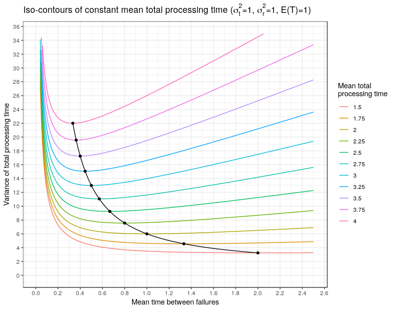
 limit; the processing time variance becomes the run-time variance. The equation also has the expected ingredients by depending on both the run-time and repair time variance. But the equation also has a bit of a surprise, it depends on the square of the mean repair time,
  . That dependence leads to an interesting trade-off.
 ,
,  , and
, and  , and fixed
  but we are free to choose
  . That is, for a given mean total processing time, we can choose between a machine that fails frequently with short repair times or we can choose a machine that fails infrequently but with long repair times. Which one would we like, and does it matter since either choice leads to the same mean total processing time? At fixed
 . But since the variance of the total processing time depends on