Improve operations: reduce variability in the queue

I recently came across a cute problem at Public Services and Procurement Canada while working on queue performance issues. Imagine a work environment where servers experience some kind of random interruption that prevents them from continuously working on a task. We’ve all been there—you’re trying to finish important work but you get interrupted by an urgent email or phone call. How can we manage this work environment? What are the possible trade-offs? Should we try to arrange for infrequent but long interruptions or should we aim for frequent but short interruptions?

Let’s rephrase the problem generically in terms of machines. Suppose that a machine processes a job in a random run-time, $T$ , with mean $\mathbb{E}(T) = \bar t$ and variance $\text{Var}(T) = \sigma_t^2$ , but with an otherwise general distribution. The machine fails with independent and identical exponentially distributed inter-arrival times. The mean time between failures is $\bar f$ . When the machine is down from failure, it takes a random amount of time, $R$ , to repair. The machine failure interrupts a job in progress and, once repaired, the machine continues the incomplete job from the point of the interruption. The repair time distribution has mean $\mathbb{E}(R) = \bar r$ and variance $\text{Var}(R) =\sigma_r^2$ but is otherwise general. The question is: What is the mean and variance of the total processing time? The solution is a bit of fun.

The time to complete a job, $\tau$ , is the sum of the (random) run-time, $T$ , plus the sum of repair times (if any). That is,

$\begin{equation*}\tau = T + \sum_{i=1}^{N(T)} R_i,\end{equation}$

where $N(T)$ is the random number of failures that occur during the run-time. First, condition $\tau$ on a run-time of $t$ and thus,

$\begin{equation*}\tau|t = t + \sum_{i=1}^{N(t)} R_i. \end{equation}$

Now, since $N(t)$ is the number of failures by time $t$ with exponentially distributed failures, this is a Poisson counting process:

$\begin{align*} \mathbb{E}(\tau|t) &= t + \mathbb{E}\left(\sum_{i=1}^{N(t)} R_i\right) \\ &= t + \sum_{k=0}^\infty \mathbb{E}\left[\left.\sum_{i=1}^k R_i \right| N(t) = k\right]\mathbb{P}(N(t) = k) \\ &= t + \sum_{k=1}^\infty (k\bar r) \frac{(t/\bar f)^k}{k!}e^{-t/\bar f} \\ & = t + \bar r \frac{t}{\bar f}e^{-t/\bar f} \sum_{k=1}^\infty \frac{(t/\bar f)^{k-1}} {(k-1)!} \\ &= t \left(\frac{\bar f + \bar r}{\bar f}\right) \end{align}$

By the law of iterated expectations, $\mathbb{E}(\mathbb{E}(\tau|t)) = \mathbb{E}(\tau)$ , and so,

$\begin{equation*} \mathbb{E}(\tau) = \mathbb{E}\left[t \left(\frac{\bar f + \bar r}{\bar f}\right)\right] = \bar t \left(\frac{\bar f + \bar r}{\bar f}\right), \end{equation}$

which gives us the mean time to process a job. Notice that in the limit that $\bar f\rightarrow\infty$ , we recover the expected result that the mean processing time is just $\mathbb{E}(T) = \bar t$ .

To derive the variance, recall the law of total variance,

$\begin{equation*}\text{Var}(Y) = \text{Var}(\mathbb{E}(Y|X))+ \mathbb{E}(\text{Var}(Y|X))\end{equation}$

From the conditional expectation calculation, we have

$\begin{equation*}\text{Var}(\mathbb{E}(\tau|t) )= \text{Var}\left[ t \left(\frac{\bar f + \bar r}{\bar f}\right)\right] = \sigma_t^2 \left(\frac{\bar f + \bar r}{\bar f}\right)^2.\end{equation}$

We need $\mathbb{E}(\text{Var}(\tau|t))$ . For fixed $t$ , we use the Laplace transform of the sum of the random repair times, $S = \sum_{i=1}^{N(t)} R_i$ , that is,

$\begin{align*} \mathcal{L}(u) = \mathbb{E}[\exp(uS)] &= \mathbb{E}\left[\exp\left(u\sum_{i=1}^{N(t)} R_i\right)\right] \\ &= \sum_{k=0}^\infty \left[(\mathcal{L}_r(u))^k | N(t) =k \right] \frac{(t/\bar f)^k}{k!}e^{-t/\bar f} \\ &= \exp\left(\frac{t}{\bar f}(\mathcal{L}_r(u) -1)\right), \end{align}$

where $\mathcal{L}_r(u)$ is the Laplace transform of the unspecified repair time distribution. The second moment is,

$\begin{equation*}\mathcal{L}^{\prime\prime}(0) = \left( \frac{t\mathcal{L}^\prime_r(0)}{\bar f}\right)^2 + \frac{t}{\bar f}\mathcal{L}^{\prime\prime}_r(0).\end{equation}$

We have the moment and variance relationships $\mathcal{L}^\prime_r(0) = \bar r$ and $\mathcal{L}^{\prime\prime}_r(0) - (\mathcal{L}^\prime_r(0))^2 = \sigma_r^2$ , and thus,

$\begin{align*} \mathbb{E}[\text{Var}(\tau|T=t)] &= \mathbb{E}[\text{Var}(t + S)|T=t] \\&= \mathbb{E}[\mathcal{L}^{\prime\prime}(0) - (\mathcal{L}^\prime(0))^2] \\ &= \mathbb{E}\left[ \left(\frac{t\bar r}{\bar f}\right)^2 + \frac{t(\sigma_r^2 + \bar r^2)}{\bar f} - \left(\frac{t\bar r}{\bar f}\right)^2 \right] \\ & = \mathbb{E}\left[\frac{t(\sigma_r^2 + \bar r^2)}{\bar f}\right] = \frac{\bar t(\sigma_r^2 + \bar r^2)}{\bar f} . \end{align}$

The law of total variance gives the desired result,

$\begin{align*} \text{Var}(\tau) &= \text{Var}(\mathbb{E}(\tau|t) ) + \mathbb{E}[\text{Var}(\tau|t)] \\ & = \left(\frac{\bar r + \bar f}{\bar f}\right)^2\sigma_t^2 + \left(\frac{\bar t}{\bar f}\right) \left(\bar r^2 + \sigma_r^2\right) \end{align}$

Notice that the equation for the total variance makes sense in the $\bar f \rightarrow \infty$ limit; the processing time variance becomes the run-time variance. The equation also has the expected ingredients by depending on both the run-time and repair time variance. But the equation also has a bit of a surprise, it depends on the square of the mean repair time, $\bar r^2$ . That dependence leads to an interesting trade-off.

Imagine that we have a setup with fixed $\sigma_t$ , $\sigma_r$ , and $\bar t$ , and fixed $\mathbb{E}(\tau)$ but we are free to choose $\bar f$ and $\bar r$ . That is, for a given mean total processing time, we can choose between a machine that fails frequently with short repair times or we can choose a machine that fails infrequently but with long repair times. Which one would we like, and does it matter since either choice leads to the same mean total processing time? At fixed $\mathbb{E}(\tau)$ we must have,

$\begin{equation*} \left(\frac{\bar f + \bar r}{\bar f}\right)=K,\end{equation}$

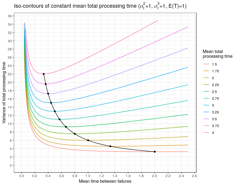
for some constant $K$ . But since the variance of the total processing time depends on $\bar r$ , different choices of $\bar f$ will lead to different total variance. The graph shows different iso-contours of constant mean total processing time in the total variance/mean time between failure plane. Along the black curve, we see that as the mean total processing time increases, we can minimize the variance by choosing a configuration where the machine fails often but with short repair times.

Minimizing total variance as a function of mean time between failures.

Why is this important? Well, in a queue, all else remaining equal, increasing server variance increases the expected queue length. So, in a workflow, if we have to live with interruptions, for the same mean processing time, it’s better to live with frequent short interruptions rather than infrequent long interruptions. The exact trade-offs depend on the details of the problem, but this observation is something that all government data scientists who are focused on improving operations should keep in the back of their mind.

Leave a Reply Cancel reply